

If you are looking for a way to perform Vegetation Index analysis using Python. This simple guide will get you started.
Carrying out Vegetation Indices analysis is a common practice in Satellite Image Processing. Geographic systems such as ENVI, ArcMap, Quantum GIS offer us a relatively straight forward way to carry out this task. However, the use of such systems could be limiting when trying to gain more control over the individual variables used in conducting Vegetation indices.
A vegetation index is a value that indicates the health and structure of vegetation biomass, it is determined by the level of reflection and absorption of light across red and near-infrared spectral bands. Most commonly healthy vegetation reflects higher in the near-infrared red (NIR) band than in the visible portion (Red band) of the Electromagnetic spectrum.
The most common type of Vegetation Indices is the Normalized Difference Vegetation Indices (NDVI). It is calculated using the following formula:
NDVI = NIR – RED/ NIR + RED
NIR is the pixel reflectance value in the near-infrared band, the RED is the pixel reflectance in the red band. NDVI values typically range from -1.0 to 1.0 for each pixel image. Most commonly dense or healthy vegetation is in the range of 0.5 – 1.0.
Let's get started.
STEP 1- DOWNLOAD SATELLITE IMAGERY
*if you already have your data, skip to step-2.*
Landsat 8 Imagery of Central Wuhan was gotten from earthexplorer.usgs.gov
Date Range: 08/01/2020 to 08/10/2020
Cloud Cover: 10%
Dataset Used: Landsat > Landsat Collection 1 level-1 > Landsat 8 OLI/TIRS C1 Level-1
STEP 2: SUBSET AND CLIP STUDY AREA
Tools used: ArcMap, Python 3.6 Jupyter Notebook
Python Packages Used: gdal, gdal.Warp , OS
Spatial Reference: WGS_84_UTM_zone_49
Landsat image data usually covers a large area, in other to ensure we focus only on our study area, a Polygon shapefile AOS.shp for the Area of Study was created in ArcMap to clip the Landsat image, the coordinate system of the polygon shapefile was set to match the coordinate system of the Landsat 8 image, this was to ensure the Clip operation runs successfully without any errors
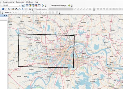 Image showing Polygon shapefile representing Area of Study
Now, this same clipping operation could be done using any GIS software but for the sake of this task, it was done using python.
To Clip the Image, gdal python library was used, the code snippet below
import gdal
import os
import rasterio as ras
from rasterio import plot
import matplotlib.pyplot as plt
import numpy as np
%matplotlib inline

#used to throw errors if there are any in the code
gdal.UseExceptions()


#filepath to downloaded spectral bands
spectralBands = '../wuhan/LandsatImages/'

#filepath to Output folder of clipped Landsat Image
outputResults = '../wuhan/Output/'

#filepath to shapefile to be used for clip operation
shpclip = '../wuhan/AOS.shp'

#creates a list of all Landsat bands ending with .TIFF in the LANDSAT image folder
bandList = [band for band in os.listdir(spectralBands) if band[-4:]=='.TIF']

#loops through the created bandlist and applies clip function gdal.warp to each individual band

for band in bandList:
    clippedFiles = outputResults + band[:-4]+'_clipped'+band[-4:]
    print(clippedFiles)
    options = gdal.WarpOptions(cutlineDSName=shpclip, cropToCutline=True)
    outBand = gdal.Warp(srcDSOrSrcDSTab=spectralBands + band,
                        destNameOrDestDS=clippedFiles, options=options)
    outBand= None
STEP 3 – CALCULATE NDVI
Tools used: ArcMap, Python 3.6 Jupyter Notebook
Python Packages Used: RASTERIO, MATPLOTLIB, NUMPY
Spatial Reference: WGS_84_UTM_zone_49
NORMALIZED DIFFERENCE VEGETATION INDEX (NDVI)
NDVI = (NIR – RED) / (NIR + RED)
After the images are successfully clipped, they are stored in an output folder specified as OutputResults in the previous code snippet. To calculate the NDVI we will use Band 4(RED band) and Band 5 (Near-Infrared), this is a standard for Landsat 8 images. Other satellite sensors use a combination of different bands e.g. sentinel-2 uses a combination of band 4 and 8
Note: If you are using Landsat 7 ETM, Band 4 is the Near-Infrared while Band 3 is the Red band. Always check for band specifications of the Satellite Sensor you’re using for your dataset.
#Calculate NDVI
#stores the band 4 and band 5 images in a variable using the file location
band4 = ras.open('../wuhan/Output/LC08_L1TP_123039_20200803_20200807_01_T1_B4_clipped.TIF')
band5 = ras.open('../wuhan/Output/LC08_L1TP_123039_20200803_20200807_01_T1_B5_clipped.TIF')


#generate nir and red objects as arrays in float64 format
red = band4.read(1).astype('float64')
nir = band5.read(1).astype('float64')

#ndvi calculation
#here, no data/empty cells are reported as 0, other values are calculated using the ndvi formula
ndvi= np.where( (nir+red)== 0, 0, (nir-red)/(nir+red) )


#exports ndvi image to a location specified with ras.open()
ndviImage = ras.open('../wuhan/Output/ndviImage.tiff', 'w', driver='Gtiff',
                          width=band4.width,
                          height = band4.height,
                          count=1, crs=band4.crs,
                          transform=band4.transform,
                          dtype='float64')

ndviImage.write(ndvi,1)
ndviImage.close()

#plot ndvi or displays the ndvi raster file
ndvi = ras.open('../wuhan/Output/ndviImage.tiff')
fig = plt.figure(figsize=(18,12))
plot.show(ndvi)
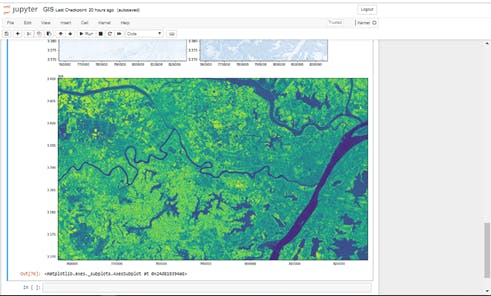 Image showing created NDVI Raster Image.
Note: In other to perform tasks such as applying a stretch, classifying your data, and symbolizing the raster data for display in ArcGIS or similar software, computing statistics on the Indices (Raster Image) is required, the ArcGIS Calculate statistics tool (Data Management) can be used for this.